Shirley K Data
Deep Learning Project
This python project explores Lending Club data to predict whether a person will pay off their loan. The data was cleaned and engineered for use with a neural network model.
Library and Data Imports
import pandas as pd
import numpy as np
import matplotlib.pyplot as plt
import seaborn as sns

%matplotlib inline
df = pd.read_csv('../DATA/lending_club_loan_two.csv')df.info()<class 'pandas.core.frame.DataFrame'>
RangeIndex: 396030 entries, 0 to 396029
Data columns (total 27 columns):
# Column Non-Null Count Dtype
--- ------ -------------- -----
0 loan_amnt 396030 non-null float64
1 term 396030 non-null object
2 int_rate 396030 non-null float64
3 installment 396030 non-null float64
4 grade 396030 non-null object
5 sub_grade 396030 non-null object
6 emp_title 373103 non-null object
7 emp_length 377729 non-null object
8 home_ownership 396030 non-null object
9 annual_inc 396030 non-null float64
10 verification_status 396030 non-null object
11 issue_d 396030 non-null object
12 loan_status 396030 non-null object
13 purpose 396030 non-null object
14 title 394275 non-null object
15 dti 396030 non-null float64
16 earliest_cr_line 396030 non-null object
17 open_acc 396030 non-null float64
18 pub_rec 396030 non-null float64
19 revol_bal 396030 non-null float64
20 revol_util 395754 non-null float64
21 total_acc 396030 non-null float64
22 initial_list_status 396030 non-null object
23 application_type 396030 non-null object
24 mort_acc 358235 non-null float64
25 pub_rec_bankruptcies 395495 non-null float64
26 address 396030 non-null object
dtypes: float64(12), object(15)
memory usage: 81.6+ MBExploratory Data Analysis
The following countplot shows the target variable distribution.
Ideally, the distribution would be more even.
sns.countplot(x='loan_status',data=df)<AxesSubplot:xlabel='loan_status', ylabel='count'>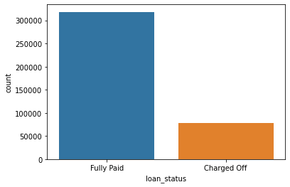
The following histogram shows the number of loans for each dollar amount.
There are noticeable peaks at each 5000th increments.
plt.figure(figsize=(12,8))
sns.histplot(df['loan_amnt'],bins=40)
<AxesSubplot:xlabel='loan_amnt', ylabel='Count'>
df.corr()| loan_amnt | int_rate | installment | annual_inc | dti | open_acc | pub_rec | revol_bal | revol_util | total_acc | mort_acc | pub_rec_bankruptcies | |
|---|---|---|---|---|---|---|---|---|---|---|---|---|
| loan_amnt | 1.000000 | 0.168921 | 0.953929 | 0.336887 | 0.016636 | 0.198556 | -0.077779 | 0.328320 | 0.099911 | 0.223886 | 0.222315 | -0.106539 |
| int_rate | 0.168921 | 1.000000 | 0.162758 | -0.056771 | 0.079038 | 0.011649 | 0.060986 | -0.011280 | 0.293659 | -0.036404 | -0.082583 | 0.057450 |
| installment | 0.953929 | 0.162758 | 1.000000 | 0.330381 | 0.015786 | 0.188973 | -0.067892 | 0.316455 | 0.123915 | 0.202430 | 0.193694 | -0.098628 |
| annual_inc | 0.336887 | -0.056771 | 0.330381 | 1.000000 | -0.081685 | 0.136150 | -0.013720 | 0.299773 | 0.027871 | 0.193023 | 0.236320 | -0.050162 |
| dti | 0.016636 | 0.079038 | 0.015786 | -0.081685 | 1.000000 | 0.136181 | -0.017639 | 0.063571 | 0.088375 | 0.102128 | -0.025439 | -0.014558 |
| open_acc | 0.198556 | 0.011649 | 0.188973 | 0.136150 | 0.136181 | 1.000000 | -0.018392 | 0.221192 | -0.131420 | 0.680728 | 0.109205 | -0.027732 |
| pub_rec | -0.077779 | 0.060986 | -0.067892 | -0.013720 | -0.017639 | -0.018392 | 1.000000 | -0.101664 | -0.075910 | 0.019723 | 0.011552 | 0.699408 |
| revol_bal | 0.328320 | -0.011280 | 0.316455 | 0.299773 | 0.063571 | 0.221192 | -0.101664 | 1.000000 | 0.226346 | 0.191616 | 0.194925 | -0.124532 |
| revol_util | 0.099911 | 0.293659 | 0.123915 | 0.027871 | 0.088375 | -0.131420 | -0.075910 | 0.226346 | 1.000000 | -0.104273 | 0.007514 | -0.086751 |
| total_acc | 0.223886 | -0.036404 | 0.202430 | 0.193023 | 0.102128 | 0.680728 | 0.019723 | 0.191616 | -0.104273 | 1.000000 | 0.381072 | 0.042035 |
| mort_acc | 0.222315 | -0.082583 | 0.193694 | 0.236320 | -0.025439 | 0.109205 | 0.011552 | 0.194925 | 0.007514 | 0.381072 | 1.000000 | 0.027239 |
| pub_rec_bankruptcies | -0.106539 | 0.057450 | -0.098628 | -0.050162 | -0.014558 | -0.027732 | 0.699408 | -0.124532 | -0.086751 | 0.042035 | 0.027239 | 1.000000 |
The following is a strong visual of which features are most correlated to one another.
plt.figure(figsize=(12,8))
sns.heatmap(df.corr(),cmap='viridis',annot=True)
<AxesSubplot:>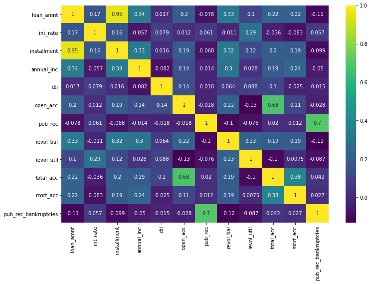
The installment amount is highly correlated to the loan amount, which makes sense.
df.columnsIndex(['loan_amnt', 'term', 'int_rate', 'installment', 'grade', 'sub_grade',
'emp_title', 'emp_length', 'home_ownership', 'annual_inc',
'verification_status', 'issue_d', 'loan_status', 'purpose', 'title',
'dti', 'earliest_cr_line', 'open_acc', 'pub_rec', 'revol_bal',
'revol_util', 'total_acc', 'initial_list_status', 'application_type',
'mort_acc', 'pub_rec_bankruptcies', 'address'],
dtype='object')grade_order = list(df['grade'].sort_values().unique())subgrade_order = list(df['sub_grade'].sort_values().unique())The following shows the number of fully paid versus charged off accounts by grade.
We see that higher grades have more instances of paid off accounts than lower grades.
sns.countplot(x='grade',data=df,hue='loan_status',order=grade_order)<AxesSubplot:xlabel='grade', ylabel='count'>
The following is what looks to be a Poisson distribution of loans by subgrade.
plt.figure(figsize=(13,5))
sns.countplot(x='sub_grade',data=df,order=subgrade_order,palette='coolwarm')
<AxesSubplot:xlabel='sub_grade', ylabel='count'>
We see in the following plot that when separated by the target variables, those with higher grades and subgrades have more instances of fully paid off loans, which is expected.
plt.figure(figsize=(13,5))
sns.countplot(x='sub_grade',data=df,order=subgrade_order,palette='coolwarm',hue='loan_status')
<AxesSubplot:xlabel='sub_grade', ylabel='count'>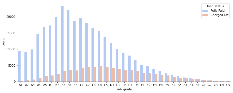
Those with F and G grades have closer to 50/50 odds of paying off their loans.
fg_df = df[(df['grade']=='F')|(df['grade']=='G')]
plt.figure(figsize=(13,5))
sns.countplot(x='sub_grade',data=fg_df,hue='loan_status',order=fg_df['sub_grade'].sort_values().unique(),palette='coolwarm')
<AxesSubplot:xlabel='sub_grade', ylabel='count'>
Feature Engineering
Prepping data for our machine learning algorithm later.
def paid_charged(pc):
    if pc == 'Fully Paid':
        return 1
    else:
        return 0
df['loan_repaid'] = df['loan_status'].apply(lambda x: paid_charged(x))df[['loan_repaid','loan_status']]| loan_repaid | loan_status | |
|---|---|---|
| 0 | 1 | Fully Paid |
| 1 | 1 | Fully Paid |
| 2 | 1 | Fully Paid |
| 3 | 1 | Fully Paid |
| 4 | 0 | Charged Off |
| ... | ... | ... |
| 396025 | 1 | Fully Paid |
| 396026 | 1 | Fully Paid |
| 396027 | 1 | Fully Paid |
| 396028 | 1 | Fully Paid |
| 396029 | 1 | Fully Paid |
396030 rows × 2 columns
Interest rate has an inverse relationship to being repaid. Annual income and mortgage accounts have a stronger correlation to a loan being repaid.
df.corr()['loan_repaid'][:-1].sort_values().plot(kind='bar')<AxesSubplot:>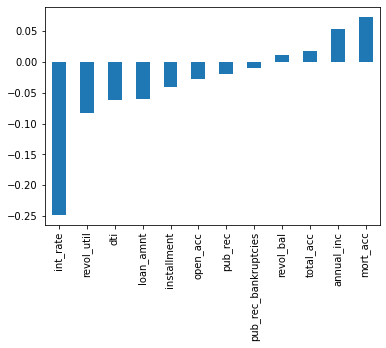
Missing Data
Missing data as percentages of the total data instances. The missing instances in Title, Revolving Utilization, and Public Record Bankruptcies are less than 1% and those instances can be deleted without impacting our dataset too much. The other three may need to have data imputed.
((df.isnull().sum())/(3960.30))loan_amnt 0.000000
term 0.000000
int_rate 0.000000
installment 0.000000
grade 0.000000
sub_grade 0.000000
emp_title 5.789208
emp_length 4.621115
home_ownership 0.000000
annual_inc 0.000000
verification_status 0.000000
issue_d 0.000000
loan_status 0.000000
purpose 0.000000
title 0.443148
dti 0.000000
earliest_cr_line 0.000000
open_acc 0.000000
pub_rec 0.000000
revol_bal 0.000000
revol_util 0.069692
total_acc 0.000000
initial_list_status 0.000000
application_type 0.000000
mort_acc 9.543469
pub_rec_bankruptcies 0.135091
address 0.000000
loan_repaid 0.000000
dtype: float64We will take a closer look at emp_title, emp_length, and mort_acc.
df['emp_title'].nunique()173105df['emp_title'].value_counts()Teacher 4389
Manager 4250
Registered Nurse 1856
RN 1846
Supervisor 1830
...
Warner Brothers 1
Liscened Practical Nirse 1
Crews Lake Middle School 1
Kaiser - Southern California Permanente 1
HIV Testing/Counseling Coordinator 1
Name: emp_title, Length: 173105, dtype: int64Employment Titles will be difficult to address effectively for our purposes. It would be hard to glean any useful and meaningful insights versus the cost to computing and time spent re-categorizing these titles. We will delete this column altogether.
df.drop('emp_title',axis=1,inplace=True)df['emp_length'].unique()array(['10+ years', '4 years', '< 1 year', '6 years', '9 years',
'2 years', '3 years', '8 years', '7 years', '5 years', '1 year',
nan], dtype=object)sorted(df['emp_length'].dropna().unique())['1 year',
'10+ years',
'2 years',
'3 years',
'4 years',
'5 years',
'6 years',
'7 years',
'8 years',
'9 years',
'< 1 year']order = ['< 1 year','1 year','2 years','3 years','4 years','5 years',
'6 years', '7 years', '8 years', '9 years','10+ years']plt.figure(figsize=(10,6))
sns.countplot(x='emp_length',data=df,order=order)<AxesSubplot:xlabel='emp_length', ylabel='count'>
What is the relationship between our target variables and this feature?
plt.figure(figsize=(10,6))
sns.countplot(x='emp_length',data=df,order=order,hue='loan_status')
<AxesSubplot:xlabel='emp_length', ylabel='count'>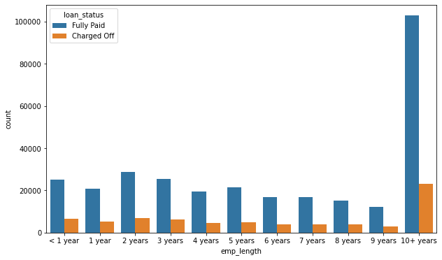
df.columnsIndex(['loan_amnt', 'term', 'int_rate', 'installment', 'grade', 'sub_grade',
'emp_length', 'home_ownership', 'annual_inc', 'verification_status',
'issue_d', 'loan_status', 'purpose', 'title', 'dti', 'earliest_cr_line',
'open_acc', 'pub_rec', 'revol_bal', 'revol_util', 'total_acc',
'initial_list_status', 'application_type', 'mort_acc',
'pub_rec_bankruptcies', 'address', 'loan_repaid'],
dtype='object')emp_co = df[df['loan_status']=="Charged Off"].groupby("emp_length").count()['loan_status']emp_fp = df[df['loan_status']=="Fully Paid"].groupby("emp_length").count()['loan_status']emp_len = emp_co/emp_fpemp_lenemp_length
1 year 0.248649
10+ years 0.225770
2 years 0.239560
3 years 0.242593
4 years 0.238213
5 years 0.237911
6 years 0.233341
7 years 0.241887
8 years 0.249625
9 years 0.250735
< 1 year 0.260830
Name: loan_status, dtype: float64emp_len.plot(kind='bar')<AxesSubplot:xlabel='emp_length'>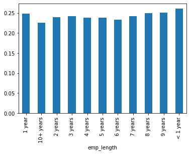
As a percentage of instances, the amount of charge off versus full repayment is consistent across employment lengths. We will drop this column as well.
df = df.drop('emp_length',axis=1)The title column is essentially the same as the purpose column. They are also both string columns.
df = df.drop('title',axis=1)df['mort_acc'].value_counts()0.0 139777
1.0 60416
2.0 49948
3.0 38049
4.0 27887
5.0 18194
6.0 11069
7.0 6052
8.0 3121
9.0 1656
10.0 865
11.0 479
12.0 264
13.0 146
14.0 107
15.0 61
16.0 37
17.0 22
18.0 18
19.0 15
20.0 13
24.0 10
22.0 7
21.0 4
25.0 4
27.0 3
23.0 2
32.0 2
26.0 2
31.0 2
30.0 1
28.0 1
34.0 1
Name: mort_acc, dtype: int64print("Correlation with the mort_acc column")
df.corr()['mort_acc'].sort_values()[:-1]Correlation with the mort_acc column
int_rate -0.082583
dti -0.025439
revol_util 0.007514
pub_rec 0.011552
pub_rec_bankruptcies 0.027239
loan_repaid 0.073111
open_acc 0.109205
installment 0.193694
revol_bal 0.194925
loan_amnt 0.222315
annual_inc 0.236320
total_acc 0.381072
Name: mort_acc, dtype: float64df.groupby('total_acc').mean()['mort_acc']total_acc
2.0 0.000000
3.0 0.052023
4.0 0.066743
5.0 0.103289
6.0 0.151293
...
124.0 1.000000
129.0 1.000000
135.0 3.000000
150.0 2.000000
151.0 0.000000
Name: mort_acc, Length: 118, dtype: float64tot_acc_avg = df.groupby('total_acc').mean()['mort_acc']tot_acc_avg[2.0]0.0The missing data will be imputed with the average value calculated by total accounts.
def fill_mort_acc(total_acc,mort_acc):
    if np.isnan(mort_acc):
        return tot_acc_avg[total_acc]
    else:
        return mort_acc
df['mort_acc'] = df.apply(lambda x: fill_mort_acc(x['total_acc'],x['mort_acc']),axis=1)We have addresssed the most significant missing data points. We can drop other missing instances since it will not impact our overall dataset significantly.
df = df.dropna()We now have no more missing data points.
df.isnull().sum()loan_amnt 0
term 0
int_rate 0
installment 0
grade 0
sub_grade 0
home_ownership 0
annual_inc 0
verification_status 0
issue_d 0
loan_status 0
purpose 0
dti 0
earliest_cr_line 0
open_acc 0
pub_rec 0
revol_bal 0
revol_util 0
total_acc 0
initial_list_status 0
application_type 0
mort_acc 0
pub_rec_bankruptcies 0
address 0
loan_repaid 0
dtype: int64Non-numeric data features.
We can now address non-number data types in our set so we can run our algorithm.
list(df.select_dtypes(exclude='number').columns)['term',
'grade',
'sub_grade',
'home_ownership',
'verification_status',
'issue_d',
'loan_status',
'purpose',
'earliest_cr_line',
'initial_list_status',
'application_type',
'address']term feature
The 'term' column can be converted to a numerical column by taking the first portion of the inputs.
df['term'][0].split()['36', 'months']df['term'] = df['term'].apply(lambda x: int(x.split()[0]))df['term'].value_counts()36 301247
60 93972
Name: term, dtype: int64grade and sub_grade features
grade is part of sub_grade, so grade is dropped.
df = df.drop('grade',axis=1)sub_grade is converted to dummy variables and the original sub_grade column is deleted.
subs = pd.get_dummies(df['sub_grade'])df.drop('sub_grade',axis=1,inplace=True)df = pd.concat([df,subs],axis=1)verification_status, application_type, initial_list_status, purpose features
Again, we will convert to dummy variables.
ver_stat = pd.get_dummies(df['verification_status'])
app_type = pd.get_dummies(df['application_type'])
init_list_stat = pd.get_dummies(df['initial_list_status'])
purp = pd.get_dummies(df['purpose'])
df = df.drop(['verification_status','application_type','initial_list_status','purpose'],axis=1)df = pd.concat([df,ver_stat,app_type,init_list_stat,purp],axis=1)list(df.select_dtypes(exclude='number').columns)['home_ownership', 'issue_d', 'loan_status', 'earliest_cr_line', 'address']home_ownership feature
df['home_ownership'].value_counts()MORTGAGE 198022
RENT 159395
OWN 37660
OTHER 110
NONE 29
ANY 3
Name: home_ownership, dtype: int64None and Any do not give us useful insights. They will be lumped together.
def home_own_type(ownership):
    if ownership.lower() in ['none','any']:
        return 'OTHER'
    else:
        return ownership

df['home_ownership'] = df['home_ownership'].apply(lambda x: home_own_type(x))
home_own_type = pd.get_dummies(df['home_ownership'])df = df.drop('home_ownership',axis=1)
df = pd.concat([df,home_own_type],axis=1)address feature
We will extract zip codes from the address column and create dummy variables.
df['address'][0][-5:]'22690'df['zip_code'] = df['address'].apply(lambda x: x[-5:])zip_codes = pd.get_dummies(df['zip_code'])
df = df.drop('zip_code',axis=1)
df = pd.concat([df,zip_codes],axis=1)df = df.drop('address',axis=1)There are three columns remaining with non-numeric data types.
df.select_dtypes(exclude='number').columnsIndex(['issue_d', 'loan_status', 'earliest_cr_line'], dtype='object')issue_d feature
issue_d is the issue date, which is not a predicting feature for our target variables. We will drop this column.
df = df.drop('issue_d',axis=1)earliest_cr_line feature
We will extract the year from the earliest_cr_line feature and use that as a numeric feature.
df['earliest_cr_line'][0][-4:]'1990'df['earliest_cr_year'] = df['earliest_cr_line'].apply(lambda x: int(x[-4:]))
df = df.drop('earliest_cr_line',axis=1)df.select_dtypes(exclude='number').columnsIndex(['loan_status'], dtype='object')Working with our Model
Train Test Split
from sklearn.model_selection import train_test_splitWe have converted loan_repaid to numeric features, so we can drop loan_status, which is essentially a repeat of those values.
df = df.drop('loan_status',axis=1)X are the features, y are the target variables.
X = df.drop('loan_repaid',axis=1).values
y = df['loan_repaid'].values
We will take a portion of our full data, due to computing resources.
df = df.sample(frac=0.1,random_state=101)
print(len(df))39522X_train, X_test, y_train, y_test = train_test_split(
X, y, test_size=0.2, random_state=101)Normalizing Data
from sklearn.preprocessing import MinMaxScalerscaler = MinMaxScaler()X_train = scaler.fit_transform(X_train)
X_test = scaler.transform(X_test)Creating Model/Neural Network
from tensorflow.keras.models import Sequential
from tensorflow.keras.layers import Dense,Dropout
from tensorflow.keras.callbacks import EarlyStoppingX_train.shape(316175, 85)We will employ early stopping to reduce time.
early_stop = EarlyStopping(monitor='val_loss',mode='auto',verbose=1,patience=25)model = Sequential()
# Input layer with rectified linear unit activation function
model.add(Dense(78,activation='relu'))
model.add(Dropout(0.5))
# Hidden layers
model.add(Dense(39,activation='relu'))
model.add(Dropout(0.5))
model.add(Dense(19,activation='relu'))
model.add(Dropout(0.5))
# Output layer with sigmoid activation function
model.add(Dense(1,activation='sigmoid'))
# Model will use adam optimizer.
model.compile(loss='binary_crossentropy',optimizer='adam')model.fit(x=X_train,y=y_train,epochs=200,
validation_data=(X_test,y_test),
verbose=1,callbacks=[early_stop])Epoch 1/200
9881/9881 [==============================] - 9s 954us/step - loss: 0.2907 - val_loss: 0.2663
Epoch 2/200
9881/9881 [==============================] - 9s 942us/step - loss: 0.2669 - val_loss: 0.2648
Epoch 3/200
9881/9881 [==============================] - 10s 962us/step - loss: 0.2659 - val_loss: 0.2640
Epoch 4/200
9881/9881 [==============================] - 9s 952us/step - loss: 0.2654 - val_loss: 0.2639
Epoch 5/200
9881/9881 [==============================] - 9s 941us/step - loss: 0.2651 - val_loss: 0.2632
Epoch 6/200
9881/9881 [==============================] - 9s 953us/step - loss: 0.2646 - val_loss: 0.2635
Epoch 7/200
9881/9881 [==============================] - 9s 952us/step - loss: 0.2644 - val_loss: 0.2625
Epoch 8/200
9881/9881 [==============================] - 10s 966us/step - loss: 0.2647 - val_loss: 0.2631
Epoch 9/200
9881/9881 [==============================] - 10s 967us/step - loss: 0.2643 - val_loss: 0.2628
Epoch 10/200
9881/9881 [==============================] - 9s 954us/step - loss: 0.2642 - val_loss: 0.2633
Epoch 11/200
9881/9881 [==============================] - 10s 970us/step - loss: 0.2642 - val_loss: 0.2634
Epoch 12/200
9881/9881 [==============================] - 10s 966us/step - loss: 0.2643 - val_loss: 0.2630
Epoch 13/200
9881/9881 [==============================] - 10s 1ms/step - loss: 0.2643 - val_loss: 0.2622
Epoch 14/200
9881/9881 [==============================] - 10s 1ms/step - loss: 0.2645 - val_loss: 0.2630
Epoch 15/200
9881/9881 [==============================] - 10s 964us/step - loss: 0.2642 - val_loss: 0.2626
Epoch 16/200
9881/9881 [==============================] - 9s 961us/step - loss: 0.2641 - val_loss: 0.2627
Epoch 17/200
9881/9881 [==============================] - 9s 954us/step - loss: 0.2638 - val_loss: 0.2634
Epoch 18/200
9881/9881 [==============================] - 10s 969us/step - loss: 0.2640 - val_loss: 0.2631
Epoch 19/200
9881/9881 [==============================] - 10s 962us/step - loss: 0.2638 - val_loss: 0.2620
Epoch 20/200
9881/9881 [==============================] - 10s 984us/step - loss: 0.2639 - val_loss: 0.2622
Epoch 21/200
9881/9881 [==============================] - 10s 973us/step - loss: 0.2635 - val_loss: 0.2623
Epoch 22/200
9881/9881 [==============================] - 9s 960us/step - loss: 0.2635 - val_loss: 0.2628
Epoch 23/200
9881/9881 [==============================] - 10s 970us/step - loss: 0.2633 - val_loss: 0.2624
Epoch 24/200
9881/9881 [==============================] - 10s 966us/step - loss: 0.2638 - val_loss: 0.2636
Epoch 25/200
9881/9881 [==============================] - 9s 959us/step - loss: 0.2637 - val_loss: 0.2629
Epoch 26/200
9881/9881 [==============================] - 10s 962us/step - loss: 0.2637 - val_loss: 0.2633
Epoch 27/200
9881/9881 [==============================] - 10s 971us/step - loss: 0.2637 - val_loss: 0.2647
Epoch 28/200
9881/9881 [==============================] - 10s 975us/step - loss: 0.2635 - val_loss: 0.2630
Epoch 29/200
9881/9881 [==============================] - 10s 967us/step - loss: 0.2631 - val_loss: 0.2623
Epoch 30/200
9881/9881 [==============================] - 9s 957us/step - loss: 0.2632 - val_loss: 0.2645
Epoch 31/200
9881/9881 [==============================] - 10s 963us/step - loss: 0.2632 - val_loss: 0.2620
Epoch 32/200
9881/9881 [==============================] - 10s 978us/step - loss: 0.2631 - val_loss: 0.2637
Epoch 33/200
9881/9881 [==============================] - 9s 959us/step - loss: 0.2633 - val_loss: 0.2630
Epoch 34/200
9881/9881 [==============================] - 10s 974us/step - loss: 0.2633 - val_loss: 0.2636
Epoch 35/200
9881/9881 [==============================] - 10s 965us/step - loss: 0.2636 - val_loss: 0.2622
Epoch 36/200
9881/9881 [==============================] - 10s 970us/step - loss: 0.2628 - val_loss: 0.2619
Epoch 37/200
9881/9881 [==============================] - 9s 961us/step - loss: 0.2627 - val_loss: 0.2629
Epoch 38/200
9881/9881 [==============================] - 10s 966us/step - loss: 0.2632 - val_loss: 0.2628
Epoch 39/200
9881/9881 [==============================] - 10s 967us/step - loss: 0.2629 - val_loss: 0.2618
Epoch 40/200
9881/9881 [==============================] - 9s 960us/step - loss: 0.2633 - val_loss: 0.2627
Epoch 41/200
9881/9881 [==============================] - 10s 962us/step - loss: 0.2630 - val_loss: 0.2625
Epoch 42/200
9881/9881 [==============================] - 9s 956us/step - loss: 0.2636 - val_loss: 0.2621
Epoch 43/200
9881/9881 [==============================] - 10s 972us/step - loss: 0.2634 - val_loss: 0.2627
Epoch 44/200
9881/9881 [==============================] - 10s 965us/step - loss: 0.2631 - val_loss: 0.2628
Epoch 45/200
9881/9881 [==============================] - 10s 964us/step - loss: 0.2632 - val_loss: 0.2622
Epoch 46/200
9881/9881 [==============================] - 10s 962us/step - loss: 0.2631 - val_loss: 0.2638
Epoch 47/200
9881/9881 [==============================] - 9s 960us/step - loss: 0.2634 - val_loss: 0.2624
Epoch 48/200
9881/9881 [==============================] - 9s 956us/step - loss: 0.2626 - val_loss: 0.2623
Epoch 49/200
9881/9881 [==============================] - 10s 968us/step - loss: 0.2632 - val_loss: 0.2627
Epoch 50/200
9881/9881 [==============================] - 10s 962us/step - loss: 0.2628 - val_loss: 0.2640
Epoch 51/200
9881/9881 [==============================] - 10s 968us/step - loss: 0.2627 - val_loss: 0.2632
Epoch 52/200
9881/9881 [==============================] - 9s 961us/step - loss: 0.2628 - val_loss: 0.2624
Epoch 53/200
9881/9881 [==============================] - 10s 967us/step - loss: 0.2631 - val_loss: 0.2618
Epoch 54/200
9881/9881 [==============================] - 9s 954us/step - loss: 0.2628 - val_loss: 0.2621
Epoch 55/200
9881/9881 [==============================] - 10s 961us/step - loss: 0.2629 - val_loss: 0.2644
Epoch 56/200
9881/9881 [==============================] - 10s 966us/step - loss: 0.2636 - val_loss: 0.2630
Epoch 57/200
9881/9881 [==============================] - 10s 966us/step - loss: 0.2635 - val_loss: 0.2623
Epoch 58/200
9881/9881 [==============================] - 9s 957us/step - loss: 0.2630 - val_loss: 0.2624
Epoch 59/200
9881/9881 [==============================] - 10s 988us/step - loss: 0.2626 - val_loss: 0.2639
Epoch 60/200
9881/9881 [==============================] - 10s 974us/step - loss: 0.2628 - val_loss: 0.2636
Epoch 61/200
9881/9881 [==============================] - 10s 965us/step - loss: 0.2631 - val_loss: 0.2628
Epoch 62/200
9881/9881 [==============================] - 10s 963us/step - loss: 0.2629 - val_loss: 0.2636
Epoch 63/200
9881/9881 [==============================] - 10s 1ms/step - loss: 0.2635 - val_loss: 0.2626
Epoch 64/200
9881/9881 [==============================] - 10s 1ms/step - loss: 0.2630 - val_loss: 0.2624
Epoch 00064: early stopping
<tensorflow.python.keras.callbacks.History at 0x7fb361785ba8>Saving this model for future use.
from tensorflow.keras.models import load_modelmodel.save('lending_club_model.h5')Evaluating Model Performance
model_loss = pd.DataFrame(model.history.history)
model_loss.plot()
<AxesSubplot:>
predictions = model.predict_classes(X_test)from sklearn.metrics import classification_report,confusion_matrixprint(confusion_matrix(y_test,predictions))
print(classification_report(y_test,predictions))[[ 6831 8827]
[ 90 63296]]
precision recall f1-score support
0 0.99 0.44 0.61 15658
1 0.88 1.00 0.93 63386
accuracy 0.89 79044
macro avg 0.93 0.72 0.77 79044
weighted avg 0.90 0.89 0.87 79044Predicting One Input
import random
random.seed(101)
random_ind = random.randint(0,len(df))

new_customer = df.drop('loan_repaid',axis=1).iloc[random_ind]
new_customer
loan_amnt 25000.00
term 36.00
int_rate 7.90
installment 782.26
annual_inc 62000.00
...
48052 0.00
70466 1.00
86630 0.00
93700 0.00
earliest_cr_year 1991.00
Name: 385487, Length: 85, dtype: float64model.predict_classes(new_customer.values.reshape(1,85))array([[1]], dtype=int32)It appears this person is likely to repay their loan.
df.iloc[random_ind]['loan_repaid']1.0They did in fact repay their loan.